Introduction to Reinforcement Learning
4 - Model-Free Prediction
| Main: | Index |
| Previous: | 3 - Planning by Dynamic Programming |
| Next: | 5 - Model-Free Control |
Introduction
Model-Free Prediction: this is when we have a problem, but we are not given an MDP and we still want to solve it. There are several methods that can be used: Monte-Carlo means we follow a trajectory of states until the end and estimates a value by looking at the samples. Another family method is Temporal-Difference learning, which can be significantly more efficient. It only looks one step ahead. These methods are at each end of a spectrum, and they can be combined in different ways, which we call the TD(λ) approach.Status on where we are:
- Last lecture. Planning by dynamic programming: Solve a known MDP
- This lecture. Model-Free prediction: estimate the value function of an unknown MDP
- Next lecture. Model-free control: optimize the value function of an unknown MDP
In model-free methods we do something similar: but now we give up on this major assumption that we know how an environment works (which is usually the case). Instead we go directly from the experience of the agent to a value function, and hence, a policy. Just like we did for DP we break it into two parts: first to evaluate policies, and then to solve for the optimal policy. The challenge is to do it without knowing the model (MDP).
Monte-Carlo Learning
Figuring out how the "world" works is quite straight forward, and MC methods are unefficient but still effective (it does solve many problems, but slowly) method and is widely used in practice. It learns from episodes of experience (so random, iterative search). MC learns from complete episodes (running a game to termination); with no bootstrapping. If we start in some state, run an episode and get 5, then start again and rerun and get 7, we simply calculate the mean and estimate the value to be 6. Caveat: only apply MC to episodic MDPs where the episodes terminate.Going into more detail. The goal is to learn vπ from episodes of experience under policy π. $$ S_1,A_1,R_2,\ldots,S_k\sim \pi $$ We are trying to learn the value function, expected future return, from any state. We look at the reward we get from each timestep and onwards. The return is the total discounted reward: $$ G_t = R_{t+1} + \gamma R_{t+2} + \ldots + \gamma^{T-1}R_T $$ Recall that the value function is the expected return: $$ v_\pi(s) = E_\pi[G_t\mid S_t = s]. $$ So, from any state, we are going to estimate the value function by calculating the mean of all returns to termination from that particular state. MC evaluation uses empirical mean return instead of expedted. There are two general approaches.
First Visit Monte-Carlo Policy evaluation.
To evaluate state s (in some loop). The first time-step t that state s is visited in an episode:
- We increment some counter: N(s) ← N(s) + 1
- We increment total return: S(s) ← S(s) + Gt
- The value is estimated by mean return: V(s) = S(s)/N(s)
- By law of large numbers: V(s)→vπ as N(s)→∞
Every Visit Monte-Carlo Policy evaluation.
A subtly different approach. For every t that state s is visited in an episode:
- We increment some counter: N(s) ← N(s) + 1
- We increment total return: S(s) ← S(s) + Gt
- The value is estimated by mean return: V(s) = S(s)/N(s)
- By law of large numbers: V(s)→vπ as N(s)→∞
Incremental mean: the mean μ1, μ2, ... of a sequence x1, x2, ... can be computed incrementally: $$ \begin{align*} \mu_k &= \frac{1}{k}\sum_{j=1}^k x_j \\ &\\ &= \frac{1}{k}\bigg(x_k + \sum_{j=1}^{k-1}x_j\bigg) \\ &\\ &= \frac{1}{k}(x_k + (k-1)\mu_{k-1}) \\ &\\ &= \frac{1}{k}(x_k + k\mu_{k-1}-\mu_{k-1}) \\ &\\ &= \mu_{k-1} + \frac{1}{k}(x_k - \mu_{k-1}) \end{align*} $$ Even though many things in the environment affects the value, we don't need to know them explicitly. We just need to calculate their effects. This is the power of RL! The incremental calculations means that we can calculate things on the fly. An interesting interpretation is that when we compare xk to μk-1 we are looking at what happened, versus what we think the mean is, then we shrink this with 1/k, and then we add it to the current previous μk-1. So when we calculate μk, we are updating it in the direction of the error we found. This idea will be repeated, and every algorithm in this lecture will take this form.
For the incremental Monte-Carlo updates: we update V(s) incrementally after episode S1, A1, R2, ..., ST. For each state St with return Gt: $$ \begin{align*} N(S_t) &= N(S_t) + 1 \\ &\\ V(S_t) &= V(S_t) + \frac{1}{N(S_t)}\Big(G_t - V(S_t)\Big) \end{align*} $$ We don't need to keep track of the value between episodes, just the visit counts. Every time we see the state, we see the "error" of what we thought the error would be, and correct the value a little bit in the direction of the error - just like we saw earlier.
In non-stationary problems, it can be useful to track a running mean, i.e. forget old episodes. $$ V(S_t) \leftarrow V(S_t) + \alpha\Big(G_t - V(S_t)\Big) $$ (In real world examples, we don't want to care about very old information)
Temporal-Difference Learning
Here we break up episodes and use incomplete returns: Temporal-Difference (TD). TD methods learn directly from episodes of experience, not from given information about the environment. It is model-free. The main difference is that we learn from incomplete episodes, by bootstrapping. TD does not rely on terminating states. In this case bootstrapping means substituting the remainder of the trajectory with an estimate of what will happen from that point onwards. In a sense, TD updates a guess towards a guess.Comparing TD and MC
The common goal is to learn vπ online from experience under policy π.
Incremental every-visit Monte-Carlo: we update value V(St) toward the actual return Gt. $$ V(S_t) \leftarrow V(S_t) + \alpha\Big(\color{red}G_t\color{black} - V(S_t)\Big) $$ In the simplest temporal-difference learning algorithm: TD(0): we update value V(St) toward estimated return Rt+1 + γV(St+1): $$ V(S_t) \leftarrow V(S_t) + \alpha\Big(\color{red}R_{t+1} + \gamma V(S_{t+1})\color{black} - V(S_t)\Big) $$
- $R_{t+1} + \gamma V(S_{t+1})$ is called the TD target
- $\delta_t = R_{t+1} + \gamma V(S_{t+1}) - V(S_t)$ is called the TD error
Advantages and Disadvantages of MC vs. TD
- TD can learn before knowing the final outcome
- TD learns online after every step
- MC must wait until the end of an episode before return is known
- TD can learn without the final outcome
- TD can learn from incomplete sequences
- MC can only earn from complete
- TD works in continuing (non-terminating) environments
- MC only works for episodic (terminating) environments
The Bias/Variance Trade-off
The return used in MC, $$ G_t = R_{t+1} + \gamma R_{t+2} + \ldots + \gamma^{T-1}R_T $$ is an unbiased estimate of vπ. The true TD target $$ R_{t+1} + \gamma v_\pi(S_{t+1}) $$ is an unbiased estimate of vπ(St). (We see this from the Bellman equation).
The TD target, which is used in practice, $$ R_{t+1} + \gamma V(S_{t+1}) $$ is a biased estimate of vπ(St). The V is based on an estimate, which is where we introduce the bias.
The benefit, is that we reduce the variance: TD target is much lower variance than the return:
- Return depends on many random actions, transitions and rewards. (See expression for Gt above)
- TD target depends on one random action, transition and reward
Further summary of the advantages/disadvantages:
- MC has high variance, zero bias
- Good convergence properties
- (Even with function approximation)
- Not very sensitive to initial value
- Very simple to understand and use
- TD has low variance, some bias
- Usually more efficient than MC
- TD(0) converges to $v_\pi(s)$
- (But not always with function approximation)
- More sensitive to initial value
As we have established, both MC and td converge: V(s)→vπ(s) as experience →∞. But what about batch solution for finite experience? Would they find the same solution? $$ \begin{align*} &s_1^1, a_1^1, r_2^1, \ldots, s_{T_1}^1 \\ &\quad\vdots \\ &s_1^K, a_1^K, r_2^K, \ldots, s_{T_1}^K \end{align*} $$ (That is, we repeatedly sample espides k∈[1, K]). We can compare them in a simple example. There are two states A, B, no discounting and 8 episodes of experience.
| A,0,B,0 |
| B, 1 |
| B, 1 |
| B, 1 |
| B, 1 |
| B, 1 |
| B, 1 |
| B, 0 |
What is V(A) and what is V(B)?
I think V(A) = 0 for both MC and TD. In MC we update the value of V(B) once everything is ended, so I'm guessing V(B) = 1. For TD we sum up and take an average, so V(B) = 6/8 = 3/4? (But I don't think this is correct! :))
Answer:
Both TD and MC will assign 3/4 to V(B). The difference is what V(A) is.
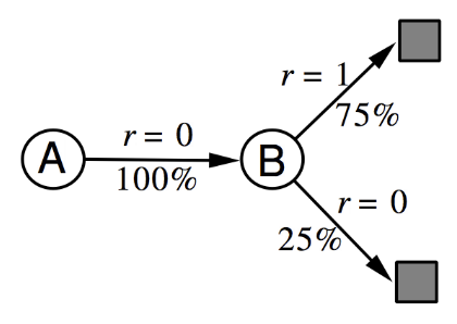
In all the episodes starting from A, we go to B and get a reward of 0. From B, 75% of the transitions gave a reward of 1, and 25% a reward of 0. This MDP gives the best description (the ML estimate) of the observed data.
MC converges to solution with minimum mean-squared error. Best fit to the observed returns: $$ \sum_{k=1}^K\sum_{t=1}^{T_k}\Big(g_t^k - V(s_t^k)\Big)^2, $$ which in the example corresponds to V(A) = 0.
TD(0) converges to solution of max likelihood Markov model. The solution to the MDP ⟨𝓢, 𝓐, 𝓟, 𝓡, 𝛾⟩ (where 𝓟 and 𝓡 are estimates): $$ \hat{\mc{P}}_{s,s'}^a = \frac{1}{N(s,a)}\sum_{k=1}^K\sum_{t=1}^{T_k}\bs{1}(s_t^k,a_t^k, s_{t+1}^k = s,a,s') $$ $$ \hat{\mc{R}}_{s}^a = \frac{1}{N(s,a)}\sum_{k=1}^K\sum_{t=1}^{T_k}\bs{1}(s_t^k,a_t^k = s,a)r_t^k, $$ which in the example corresponds to V(A) = 0.75. The probability is simply counting all episodes that go from s to s' and divide by the number of visits to s. And the reward is the average observed reward.
The third kind of Advantage/Disadvantage.
- TD exploits Markov property
- Usually more efficient in Markov environments
- MC does not exploit Markov property
- Usually more efficient in non-Markov environments