Introduction to Reinforcement Learning

3 - Planning by Dynamic Programming

Main:	Index
Previous:	3 - Planning by Dynamic Programming
Next:	4 - Model-Free Prediction

Value Iteration

Just to refresh the basic principle of dynamic programming (DP) which is the principle of optimality. Any optimal policy can be subdivided into two components:

• An optimal first action A_*...
• ...Followed by an optimal policy from successor state S'.

Following an optimal course simply means performing the optimal action from any given state. This is formalized in the following Theorem.


More informally: a policy is optimal only if for each state me might end up in, the policy would behave optimally from that state onwards. And this is a requirement for optimality.

We will use this to build a value iteration algorithm. Think of the value function as a caching our solutions to all of our subproblems. When we end up in some state, we simply assume we know the optimal solution (like if someone had told us what v_*(s') was.)

If we know the solution to subproblems v_*(s'), then the solution v_*(s) can be found by one-step lookahead: $$ v_*(s)\leftarrow \max_{a\in\mc{A}}\mc{R}_s^a + \gamma\sum_{s'\in\mc{S}}\mc{P}_{ss'}^a v_*(s') $$ We assume we know the optimal value in the "leaves", and then collect all information and put it in the "root node". The idea of value iteration, is to apply these updates iteratively. We start with some random values, and then find better values through iteration.

Intuitively: we start at the end of the problem with the final rewards, and work our way backwards. We start at the end and work our way backwards until we have discovered the optimal path; so we loop over our entire state space. (Still works with loopy, stochstic MDPs).

Simple example, with another grid world where we want to solve a shortest path problem to the colored cell and we can only move {n, e, s, w} and -1 reward per step.



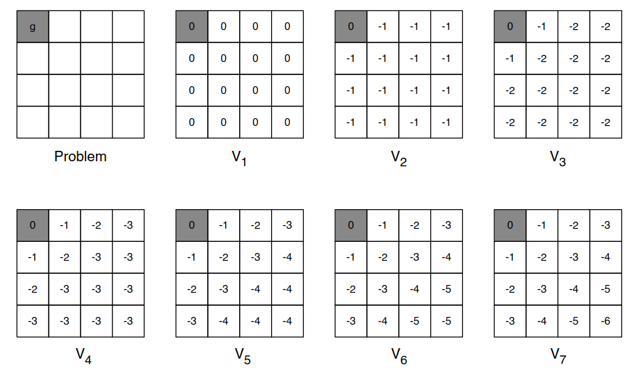
We initialize with 0s. After second iteration we have mapped -1s and so forth. The values propogate through, and we are able to find the optimal value function in every cell.

Now, a more general view of value iteration. The problem is that we want to find an optimal policy π of some MDP. And we are not solving the full RL problem, because we are being told what the dynamics of the system is, how the environment works, and we are being told what the rewards are. So we are just solving the planning. We looked at policy iteration - and value iteration is just another mechanism of solving it.

So to find the optimal policy with value iteration, is with an iterative application of Bellman optimality backup. Earlier we used the expectation variant to evaluate a specific policy, but now we find the optimal value function: $$ v_1 \rightarrow v_2 \rightarrow \ldots \rightarrow v_* $$ We use synchronous backups:
At each iteration k+1, for all states s∈𝓢, we update v_k+1(s) from v_k(s').

Convergence will be proven later with contraction mapping. Now, unlike policy iteration, we are not building a policy in every iteration: there is no explicit policy. Intermediate value functions may not correspond to any policy, but the end result will correspond to the optimal policy. Going back to the policy iteration example: there we calculated the values, then we made a greedy policy. In value iteration, we don't make the policy, but just work on the numbers.

Summary of DP algorithms: $$ \begin{array}{|l|l|l|} \hline \textbf{Problem} & \textbf{Bellman Equation} & \textbf{Algorithm} \\ \hline \text{Prediction} & \text{Bellman Expectation Equation} & \text{Iterative Policy Evaluation} \\ \hline \text{Control} & \text{Bellman Exp. Equation + Greedy Policy Impr.} & \text{Policy Evaluation} \\ \hline \text{Control} & \text{Bellman Optimality Equation} & \text{Value Iteration} \\ \hline \end{array} $$ There are different problems we want to solve - and all of them are planning problems. The MDP is given and we want to solve it. There are two types: prediction and control. For prediction we want calculate how much reward we get for som given policy. We use the Bellman expectation equation which is turned into an iterative policy evaluation. In control (two different ways), which is how to find the total reward, or optimal policy. Now we use the Bellman expectation equation with a greedy policy improvement, or a Bellman optimality equation.

All these algorithms are based on state-value functions, $v_\pi(s)$ or $v_*(s)$. Complexity is O(mn²) per iteration for m actions and n states. This could also apply to action-value functions $q_\pi(s,a)$ or $q_*(s,a)$, for which the complexity would be O(m²n²).

Extensions to Dynamic Programming

Perhaps later...

Contraction Mapping

Perhaps later...