Chapter 2 - Continuous Probability Densities

2.1 Simulation of Continuous Probabilities

Main:	Index
Previous:	1.2 Discrete Probability Distributions
Next:	2.2 Continuous Density Functions

Exercise 1

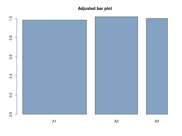
In the spinner problem (see Example 2.1) divide the unit circumference into three arcs of length 1/2, 1/3, and 1/6. Write a program to simulate the spinner experiment 1000 times and print out what fraction of the outcomes fall in each of the three arcs. Now plot a bar graph whose bars have width 1/2, 1/3, and 1/6, and areas equal to the corresponding fractions as determined by your simulation. Show that the heights of the bars are all nearly the same.

Answer

Result:

Code
Output

> A1;A2;A3
[1] 0.493
[1] 0.34
[1] 0.167

Exercise 2

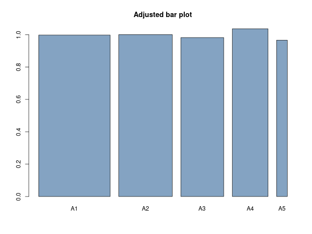
Do the same as in Exercise 1, but divide the unit circumference into five arcs of length 1/3, 1/4, 1/5, 1/6, and 1/20.

Answer

Result:

Code
Output

> A1;A2;A3;A4;A5
[1] 0.3325
[1] 0.2501
[1] 0.1964
[1] 0.1727
[1] 0.0483

Exercise 3

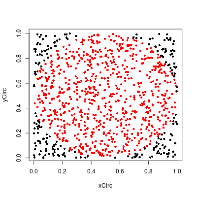
Alter the program MonteCarlo to estimate the area of the circle of radius 1/2 with center at (1/2, 1/2) inside the unit square by choosing 1000 points at random. Compare your results with the true value of π/4. Use your results to estimate the value of π. How accurate is your estimate?

Answer

Did a few simulations and the estimate for $\pi$ varied a bit. One good simulation gave 3.156. This could be made better by increasing the number of simulated points.

Code
Output

> hit/1000
[1] 0.789
> #pi
> 4*hit/1000
[1] 3.156

Exercise 4

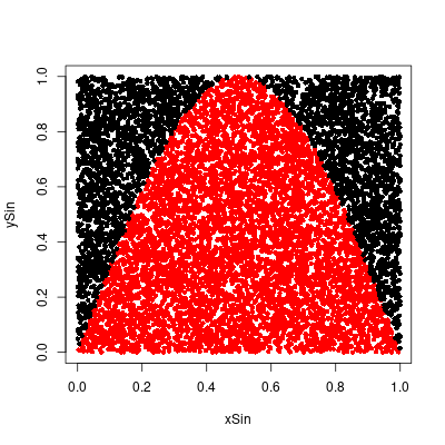
Alter the program MonteCarlo to estimate the area under the graph of $y = \sin \pi x$ inside the unit square by choosing 10,000 points at random. Now calculate the true value of this area and use your results to estimate the value of π. How accurate is your estimate?

Answer
Calculating the true value of the area in the interval [0, 1]. \begin{align} \int_0^1\sin(\pi x)dx &= \left[-\frac{1}{\pi}\cos(\pi x)\right]_0^1 \\ &= -\frac{1}{\pi}\cos(\pi) + \frac{1}{\pi}\cos(0) \\ &= \frac{1}{\pi} + \frac{1}{\pi} \\ &= \frac{2}{\pi} \end{align} The estimate for $2/\pi$ is quite close and the estimate for $\pi$ is around 3.137747.

Code
Output

> # 2/pi
> hit/NVALS
[1] 0.6374
> 2/pi
[1] 0.6366198
> (hit/NVALS)/(2/pi)
[1] 1.001226
> 
> # pi
> 2/(hit/NVALS)
[1] 3.137747

Exercise 5

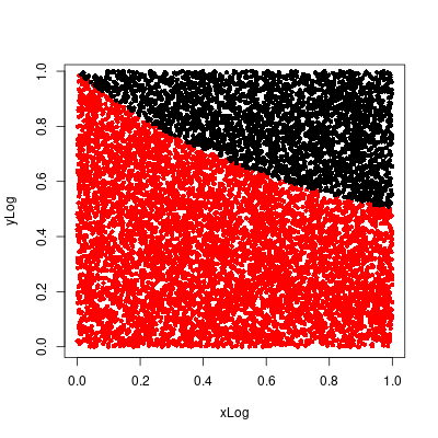
Alter the program MonteCarlo to estimate the area under the graph of $y = 1/(x + 1)$ in the unit square in the same way as in Exercise 4. Calculate the true value of this area and use your simulation results to estimate the value of $\ln 2$. How accurate is your estimate?

Answer

Calculating the true value. \begin{align} \int_0^1 \frac{1}{x + 1}dx &= \Big[\ln(x + 1)\Big]_0^1 \\ &= \ln(2) - \ln(1) \\ &= \ln(2) \\ &\approx 0.6931472 \end{align} Estimated value is 0.6939, which is close to the approximated true value, 0.6931472. As shown below the simulated estimate is within 0.1% of the true value.

Code
Output

> # log(2)
> hit/NVALS
[1] 0.6939
> log(2)
[1] 0.6931472
> (hit/NVALS)/log(2)
[1] 1.001086

Exercise 6

To simulate the Buffon’s needle problem we choose independently the distance d and the angle $\theta$ at random, with $0 \leq d \leq 1/2$ and $0 \leq \theta \leq \pi/2$, and check whether $d \leq (1/2)\sin\theta$. Doing this a large number of times, we estimate $\pi$ as $2/a$, where $a$ is the fraction of the times that $d \leq (1/2)\sin\theta$. Write a program to estimate $\pi$ by this method. Run your program several times for each of 100, 1000, and 10,000 experiments. Does the accuracy of the experimental approximation for $\pi$ improve as the number of experiments increases?

Answer
The approximation for $\pi$ does become closer on average, but it is still quite unstable. Sometimes a simulation with 1.000.000 performed worse than a simulation with 10.000 experiments.

Code
Output

> simBuffon(100)
[1] 3.389831
> simBuffon(1000)
[1] 3.12989
> simBuffon(10000)
[1] 3.137255
> simBuffon(100000)
[1] 3.13952
> simBuffon(1000000)
[1] 3.143656

Exercise 7

For Buffon’s needle problem, Laplace considered a grid with horizontal and vertical lines one unit apart. He showed that the probability that a needle of length L ≤ 1 crosses at least one line is $$ p = \frac{4L - L^2}{\pi} $$ To simulate this experiment we choose at random an angle $\theta$ between 0 and $\pi/2$ and independently two numbers $d_1$ and $d_2$ between 0 and L/2. (The two numbers represent the distance from the center of the needle to the nearest horizontal and vertical line.) The needle crosses a line if either $d_1 \leq (L/2)\sin\theta$ or $d_2 \leq (L/2)\cos\theta$. We do this a large number of times and estimate $\pi$ as $$ \overline{\pi} = \frac{4L - L^2}{a} $$ where a is the proportion of times that the needle crosses at least one line. Write a program to estimate $\pi$ by this method, run your program for 100, 1000, and 10,000 experiments, and compare your results with Buffon’s method described in Exercise 6. (Take L = 1.)

Answer
The estimates for $\pi$ appear to be quite a lot closer with the Laplace method, especially for smaller values of $n$.

Code
Output

> simLaplace(100)
[1] 3.061224
> simLaplace(1000)
[1] 3.10559
> simLaplace(10000)
[1] 3.143666
> simLaplace(100000)
[1] 3.141789
> simLaplace(1000000)
[1] 3.142694

Exercise 8

A long needle of length L much bigger than 1 is dropped on a grid with horizontal and vertical lines one unit apart. We will see (in Exercise 6.3.28) that the average number $a$ of lines crossed is approximately $$ a = \frac{4L}{\pi} $$ To estimate π by simulation, pick an angle θ at random between 0 and π/2 and compute $L\sin\theta + L\cos\theta$. This may be used for the number of lines crossed. Repeat this many times and estimate π by $$ \overline{\pi} = \frac{4L}{a} $$ where a is the average number of lines crossed per experiment. Write a program to simulate this experiment and run your program for the number of experiments equal to 100, 1000, and 10,000. Compare your results with the methods of Laplace or Buffon for the same number of experiments. (Use L = 100.)

Answer
The estimates are even closer to $\pi$, with the result for 1.000.000 experiments falls within 0.0001% of $\pi$. That's pretty close!

Code
Output

> simLongNeedle(100)
[1] 3.13445
> simLongNeedle(1000)
[1] 3.14688
> simLongNeedle(10000)
[1] 3.143391
> simLongNeedle(100000)
[1] 3.140012
> simLongNeedle(1000000)
[1] 3.141351
> pi
[1] 3.141593
> pi/3.141351
[1] 1.000077

Exercise 9

Skipped. Poorly formulated exercise.

Exercise 10

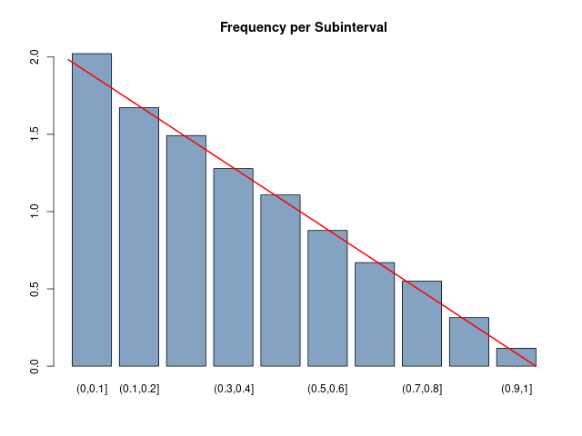
In this problem, we will again consider an experiment whose outcomes are not equally likely. We will determine a function $f(x)$ which can be used to determine the probability of certain events. Let T be the right triangle in the plane with vertices at the points (0, 0), (1, 0), and (0, 1). The experiment consists of picking a point at random in the interior of T , and recording only the x-coordinate of the point. Thus, the sample space is the set [0, 1], but the outcomes do not seem to be equally likely. We can simulate this experiment by asking a computer to return two random real numbers in [0, 1], and recording the first of these two numbers if their sum is less than 1. Write this program and run it for 10,000 trials. Then make a bar graph of the result, breaking the interval [0, 1] into 10 intervals. Compare the bar graph with the function $f(x) = 2 − 2x$. Now show that there is a constant c such that the height of T at the x-coordinate value x is c times f (x) for every x in [0, 1]. Finally, show that $$ \int_0^1 f(x) dx = 1 $$ How might one use the function $f(x)$ to determine the probability that the outcome is between 0.2 and 0.5?

Answer

Code
Output

Exercise 11

Here is another way to pick a chord at random on the circle of unit radius. Imagine that we have a card table whose sides are of length 100. We place coordinate axes on the table in such a way that each side of the table is parallel to one of the axes, and so that the center of the table is the origin. We now place a circle of unit radius on the table so that the center of the circle is the origin. Now pick out a point $(x_0 , y_0)$ at random in the square, and an angle θ at random in the interval (−π/2, π/2). Let $m = \tan\theta$. Then the equation of the line passing through $(x_0 , y_0)$ with slope m is $$ y = y_0 + m(x - x_0) $$ and the distance of this line from the center of the circle (i.e., the origin) is $$ d = \left|\frac{y_0 - mx_0}{\sqrt{m^2 + 1}}\right| $$ We can use this distance formula to check whether the line intersects the circle (i.e., whether d < 1). If so, we consider the resulting chord a random chord.

This describes an experiment of dropping a long straw at random on a table on which a circle is drawn.

Write a program to simulate this experiment 10.000 times and estimate the probability that the length of the chord is greater than $\sqrt{3}$. How does your estimate compare with the results of Example 2.6?

Answer

This experiment gives a fourth interpretation, since the proportion of chords of length larger than $\sqrt{3}$ is about 0.577 (and quite consistently). Presumably, this represents a separate interpretation.

Code
Output

> res = simChord(10000)
> res
[1] 0.5779924